TimeDB Quickstart
TimeDB is a thin ClickHouse client for 3-dimensional time series. Every value carries a valid_time (the wall-clock timestamp it describes) and a knowledge_time (when the value was learned). That makes it trivial to store forecast revisions, audit corrections, and reconstruct what was known at any past instant.
This quickstart walks through the full 3-dimensional model:
Setup
Insert a forecast and read it back
Insert a revised forecast — see the latest value win
Read the full version history
Visualize how forecast revisions evolved
Correct an erroneous value (immutable storage; corrections are new rows)
Audit the correction trail
1. Setup
TimeDBClient reads connection settings from TIMEDB_CH_URL. Series identity is supplied externally — TimeDB itself stores no metadata, only events keyed by series_id.
[1]:
try:
    import urllib.request
    import google.colab  # noqa: F401

    urllib.request.urlretrieve(
        "https://raw.githubusercontent.com/rebase-energy/timedb/main/examples/colab_setup.py", "/tmp/colab_setup.py"
    )
    exec(open("/tmp/colab_setup.py").read())
except ImportError:
    pass
[2]:
from datetime import UTC, datetime, timedelta

import polars as pl
from timedb import TimeDBClient

td = TimeDBClient()
td.delete()
td.create()
print("schema ready")

# Series identity is owned upstream (e.g. by energydb). For this demo we just
# pick an integer.
SERIES_ID = 1
base_vt = datetime(2026, 1, 1, tzinfo=UTC)
schema ready
2. Insert a forecast
The dataframe needs series_id, valid_time, and value. retention (short / medium / long) chooses the TTL tier and knowledge_time stamps when the forecast was issued.
[3]:
def make_forecast(kt: datetime, bias: float, n: int = 24) -> pl.DataFrame:
    return pl.DataFrame(
        {
            "series_id": [SERIES_ID] * n,
            "valid_time": [base_vt + timedelta(hours=i) for i in range(n)],
            "value": [50.0 + bias + 0.5 * i for i in range(n)],
        }
    )


kt_run1 = base_vt - timedelta(hours=12)
df_run1 = make_forecast(kt_run1, bias=0.0)

td.write(df_run1, retention="medium", knowledge_time=kt_run1)
print(f"wrote {df_run1.height} rows  knowledge_time={kt_run1}")
wrote 24 rows knowledge_time=2025-12-31 12:00:00+00:00
3. Insert a revised forecast
Six hours later the producer issues a corrected forecast for the same valid_time window. TimeDB doesn’t overwrite anything — both runs are kept.
[4]:
kt_run2 = base_vt - timedelta(hours=6)
df_run2 = make_forecast(kt_run2, bias=2.5)

td.write(df_run2, retention="medium", knowledge_time=kt_run2)
print(f"wrote {df_run2.height} rows  knowledge_time={kt_run2}")
wrote 24 rows knowledge_time=2025-12-31 18:00:00+00:00
4. Read the latest forecast
read() returns one row per valid_time — always the most recently issued forecast (highest knowledge_time). Run 2 wins for every hour.
[5]:
latest = td.read(series_ids=[SERIES_ID])
print(f"{latest.height} rows (one per valid_time)")
print(latest)
24 rows (one per valid_time)
shape: (24, 3)
┌───────────┬─────────────────────────┬───────┐
│ series_id ┆ valid_time              ┆ value │
│ ---       ┆ ---                     ┆ ---   │
│ u64       ┆ datetime[μs, UTC]       ┆ f64   │
╞═══════════╪═════════════════════════╪═══════╡
│ 1         ┆ 2026-01-01 00:00:00 UTC ┆ 52.5  │
│ 1         ┆ 2026-01-01 01:00:00 UTC ┆ 53.0  │
│ 1         ┆ 2026-01-01 02:00:00 UTC ┆ 53.5  │
│ 1         ┆ 2026-01-01 03:00:00 UTC ┆ 54.0  │
│ 1         ┆ 2026-01-01 04:00:00 UTC ┆ 54.5  │
│ …         ┆ …                       ┆ …     │
│ 1         ┆ 2026-01-01 19:00:00 UTC ┆ 62.0  │
│ 1         ┆ 2026-01-01 20:00:00 UTC ┆ 62.5  │
│ 1         ┆ 2026-01-01 21:00:00 UTC ┆ 63.0  │
│ 1         ┆ 2026-01-01 22:00:00 UTC ┆ 63.5  │
│ 1         ┆ 2026-01-01 23:00:00 UTC ┆ 64.0  │
└───────────┴─────────────────────────┴───────┘
5. Read the full revision history
include_knowledge_time=True returns one row per (series_id, knowledge_time, valid_time) — every forecast run side-by-side.
[6]:
history = td.read(series_ids=[SERIES_ID], include_knowledge_time=True)
print(f"{history.height} rows across {history['knowledge_time'].n_unique()} runs")
print(history)
48 rows across 2 runs
shape: (48, 4)
┌───────────┬─────────────────────────┬─────────────────────────┬───────┐
│ series_id ┆ knowledge_time          ┆ valid_time              ┆ value │
│ ---       ┆ ---                     ┆ ---                     ┆ ---   │
│ u64       ┆ datetime[μs, UTC]       ┆ datetime[μs, UTC]       ┆ f64   │
╞═══════════╪═════════════════════════╪═════════════════════════╪═══════╡
│ 1         ┆ 2025-12-31 12:00:00 UTC ┆ 2026-01-01 00:00:00 UTC ┆ 50.0  │
│ 1         ┆ 2025-12-31 18:00:00 UTC ┆ 2026-01-01 00:00:00 UTC ┆ 52.5  │
│ 1         ┆ 2025-12-31 12:00:00 UTC ┆ 2026-01-01 01:00:00 UTC ┆ 50.5  │
│ 1         ┆ 2025-12-31 18:00:00 UTC ┆ 2026-01-01 01:00:00 UTC ┆ 53.0  │
│ 1         ┆ 2025-12-31 12:00:00 UTC ┆ 2026-01-01 02:00:00 UTC ┆ 51.0  │
│ …         ┆ …                       ┆ …                       ┆ …     │
│ 1         ┆ 2025-12-31 18:00:00 UTC ┆ 2026-01-01 21:00:00 UTC ┆ 63.0  │
│ 1         ┆ 2025-12-31 12:00:00 UTC ┆ 2026-01-01 22:00:00 UTC ┆ 61.0  │
│ 1         ┆ 2025-12-31 18:00:00 UTC ┆ 2026-01-01 22:00:00 UTC ┆ 63.5  │
│ 1         ┆ 2025-12-31 12:00:00 UTC ┆ 2026-01-01 23:00:00 UTC ┆ 61.5  │
│ 1         ┆ 2025-12-31 18:00:00 UTC ┆ 2026-01-01 23:00:00 UTC ┆ 64.0  │
└───────────┴─────────────────────────┴─────────────────────────┴───────┘
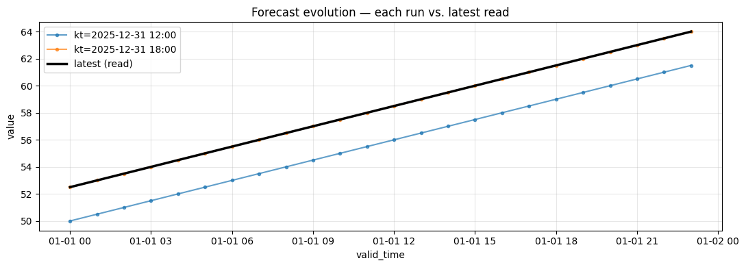
6. Visualize the 3-dimensional evolution
Each line is one forecast run; runs issued closer to the valid window converge toward the truth. The thick black line is what read() returns — the latest available value per valid_time.
[7]:
import matplotlib.pyplot as plt

fig, ax = plt.subplots(figsize=(11, 4))
for kt, run_df in history.sort("valid_time").group_by("knowledge_time", maintain_order=True):
    ax.plot(
        run_df["valid_time"].to_list(),
        run_df["value"].to_list(),
        marker="o",
        markersize=3,
        alpha=0.7,
        label=f"kt={kt[0].strftime('%Y-%m-%d %H:%M')}",
    )

latest_sorted = latest.sort("valid_time")
ax.plot(
    latest_sorted["valid_time"].to_list(),
    latest_sorted["value"].to_list(),
    color="black",
    linewidth=2.5,
    label="latest (read)",
    zorder=10,
)

ax.set_xlabel("valid_time")
ax.set_ylabel("value")
ax.set_title("Forecast evolution — each run vs. latest read")
ax.legend(loc="upper left")
ax.grid(True, alpha=0.3)
plt.tight_layout()
plt.show()
7. Correct an erroneous value
ClickHouse is append-only, so corrections are just new rows with a later knowledge_time. Suppose hours 10–12 of run 2 had a sensor glitch. We re-write only those three rows with a fresh knowledge_time and the corrected values.
[8]:
correction_kt = base_vt
hours_to_fix = [10, 11, 12]

correction = pl.DataFrame(
    {
        "series_id": [SERIES_ID] * len(hours_to_fix),
        "valid_time": [base_vt + timedelta(hours=h) for h in hours_to_fix],
        # Replace the buggy values with something sensible
        "value": [60.0, 61.0, 62.0],
    }
)
td.write(correction, retention="medium", knowledge_time=correction_kt)
print(f"correction issued at kt={correction_kt}  ({correction.height} rows)")
correction issued at kt=2026-01-01 00:00:00+00:00 (3 rows)
8. Verify the correction won — and audit the trail
read() shows the corrected values at hours 10–12. The full history still preserves every prior version.
[9]:
latest = td.read(series_ids=[SERIES_ID]).sort("valid_time")
window = latest.filter(pl.col("valid_time").is_between(base_vt + timedelta(hours=9), base_vt + timedelta(hours=13)))
print("Latest values around the corrected window:")
print(window)
Latest values around the corrected window:
shape: (5, 3)
┌───────────┬─────────────────────────┬───────┐
│ series_id ┆ valid_time              ┆ value │
│ ---       ┆ ---                     ┆ ---   │
│ u64       ┆ datetime[μs, UTC]       ┆ f64   │
╞═══════════╪═════════════════════════╪═══════╡
│ 1         ┆ 2026-01-01 09:00:00 UTC ┆ 57.0  │
│ 1         ┆ 2026-01-01 10:00:00 UTC ┆ 60.0  │
│ 1         ┆ 2026-01-01 11:00:00 UTC ┆ 61.0  │
│ 1         ┆ 2026-01-01 12:00:00 UTC ┆ 62.0  │
│ 1         ┆ 2026-01-01 13:00:00 UTC ┆ 59.0  │
└───────────┴─────────────────────────┴───────┘
[10]:
history = td.read(series_ids=[SERIES_ID], include_knowledge_time=True).sort(["valid_time", "knowledge_time"])
audit = history.filter(pl.col("valid_time").is_between(base_vt + timedelta(hours=9), base_vt + timedelta(hours=13)))
print("Full audit — every (knowledge_time, valid_time) pair:")
print(audit)
Full audit — every (knowledge_time, valid_time) pair:
shape: (13, 4)
┌───────────┬─────────────────────────┬─────────────────────────┬───────┐
│ series_id ┆ knowledge_time          ┆ valid_time              ┆ value │
│ ---       ┆ ---                     ┆ ---                     ┆ ---   │
│ u64       ┆ datetime[μs, UTC]       ┆ datetime[μs, UTC]       ┆ f64   │
╞═══════════╪═════════════════════════╪═════════════════════════╪═══════╡
│ 1         ┆ 2025-12-31 12:00:00 UTC ┆ 2026-01-01 09:00:00 UTC ┆ 54.5  │
│ 1         ┆ 2025-12-31 18:00:00 UTC ┆ 2026-01-01 09:00:00 UTC ┆ 57.0  │
│ 1         ┆ 2025-12-31 12:00:00 UTC ┆ 2026-01-01 10:00:00 UTC ┆ 55.0  │
│ 1         ┆ 2025-12-31 18:00:00 UTC ┆ 2026-01-01 10:00:00 UTC ┆ 57.5  │
│ 1         ┆ 2026-01-01 00:00:00 UTC ┆ 2026-01-01 10:00:00 UTC ┆ 60.0  │
│ …         ┆ …                       ┆ …                       ┆ …     │
│ 1         ┆ 2025-12-31 12:00:00 UTC ┆ 2026-01-01 12:00:00 UTC ┆ 56.0  │
│ 1         ┆ 2025-12-31 18:00:00 UTC ┆ 2026-01-01 12:00:00 UTC ┆ 58.5  │
│ 1         ┆ 2026-01-01 00:00:00 UTC ┆ 2026-01-01 12:00:00 UTC ┆ 62.0  │
│ 1         ┆ 2025-12-31 12:00:00 UTC ┆ 2026-01-01 13:00:00 UTC ┆ 56.5  │
│ 1         ┆ 2025-12-31 18:00:00 UTC ┆ 2026-01-01 13:00:00 UTC ┆ 59.0  │
└───────────┴─────────────────────────┴─────────────────────────┴───────┘
Summary
Concept |
Description |
|---|---|
|
The timestamp the value describes |
|
When the value was learned |
|
Append rows; corrections are just new rows with a later |
|
Latest value per |
|
Every |
For richer hierarchies (sites, assets, edges, units, runs metadata) use `energydb <../../energydb/examples/quickstart.ipynb>`__ on top.